How to Choose Preprocessing Methods: MinMaxScaler, StandardScaler, RobustScaler, and Normalizer

Preprocessing is often not optional in machine learning. When feature scales differ a lot, or when a dataset contains noticeable outliers, the choice of scaling method can directly affect model behavior.

In sklearn, the most common names around this topic are MinMaxScaler, StandardScaler, RobustScaler, and Normalizer. They all sound like “normalization”, but they are not doing the same thing.

This article first separates the concepts, then uses a small simulated dataset to show what changes after each transformation, and finally gives a more practical selection guide.

Definitions

It helps to separate the common terms first:

• scale: a broad term meaning that you change the numeric scale of the data
• standardize: usually means subtracting the mean and dividing by the standard deviation, so the transformed feature has mean near 0 and standard deviation near 1
• normalize: often used loosely in articles, but in sklearn, Normalizer has a more specific meaning: it rescales each sample to unit norm

So StandardScaler, MinMaxScaler, and RobustScaler usually operate feature by feature, while Normalizer usually operates sample by sample.

A quick selection rule

If you only want a quick rule of thumb, use this order:

1. If feature scales differ a lot and outliers are not the main problem, start with StandardScaler
2. If you need values compressed into a fixed range such as [0, 1], consider MinMaxScaler
3. If outliers are obvious, check RobustScaler
4. If the direction of each sample vector matters more than the absolute size, such as text vectors or cosine similarity workflows, look at Normalizer

Why?

Why does preprocessing matter at all?

Because many algorithms are sensitive to feature scale. If one feature has values in the thousands while another stays near 0 or 1, the model may overemphasize the larger-scale feature.

Algorithms that are often noticeably affected include:

• Linear Regression
• KNN (K-Nearest Neighbors)
• Neural Networks (NN)
• Support Vector Machines (SVM)
• PCA (Principal Component Analysis)
• LDA (Linear Discriminant Analysis)

Distance-based methods, gradient-based methods, and variance-based transformations are especially sensitive to this issue.

Generating Test Data

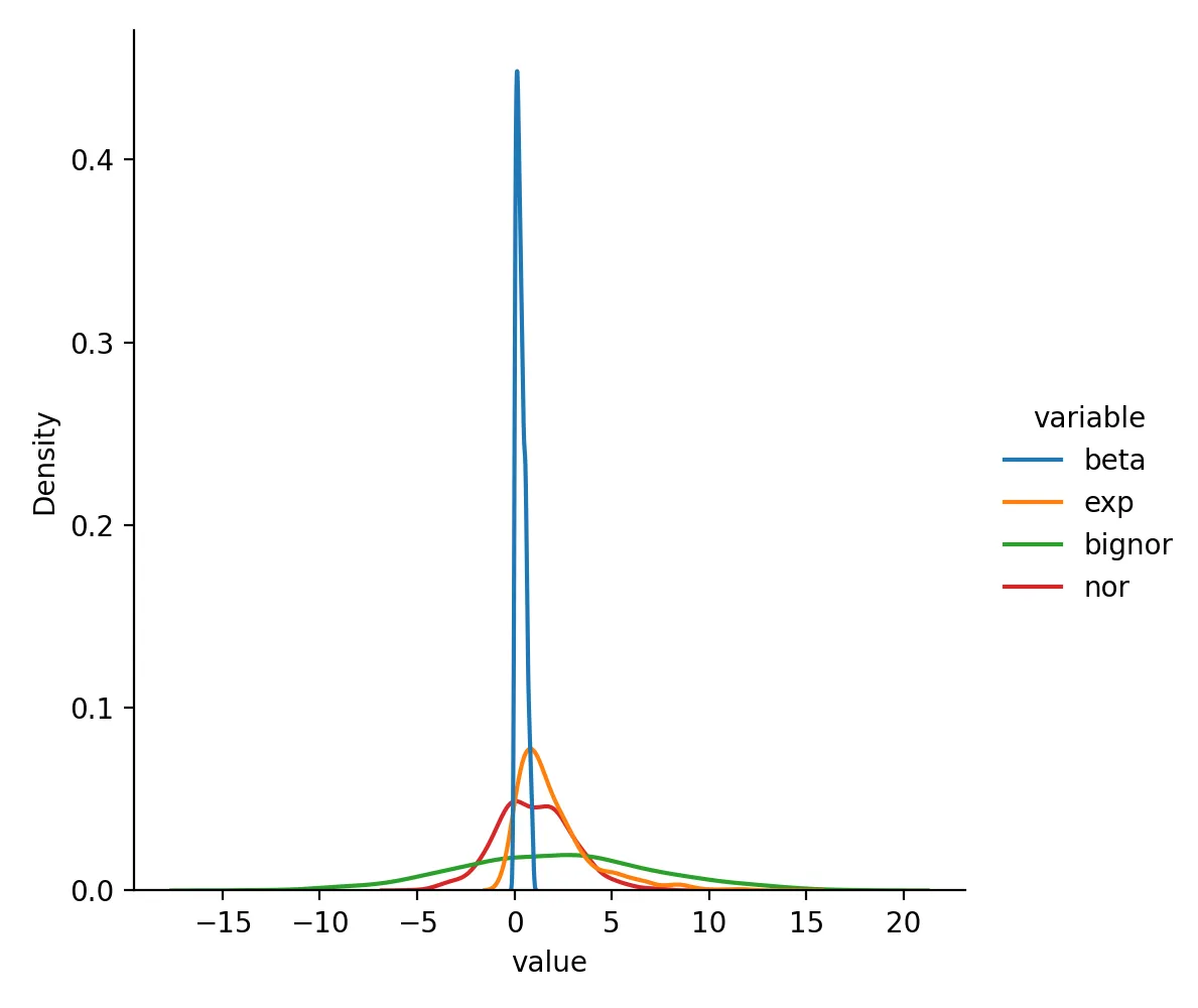
Below we generate a small simulated dataset with a beta distribution, an exponential distribution, a normal distribution, and another normal distribution with larger spread. This makes it easier to see how different preprocessing methods behave.

import numpy as np
import pandas as pd
import matplotlib.pyplot as plt
import seaborn as sns

# Set seed to ensure reproducibility
np.random.seed(1024)
data_beta = np.random.beta(1, 2, 1000)
data_exp = np.random.exponential(scale=2, size=1000)
data_nor = np.random.normal(loc=1, scale=2, size=1000)
data_bignor = np.random.normal(loc=2, scale=5, size=1000)

# Create dataframe
df = pd.DataFrame({
    "beta": data_beta,
    "exp": data_exp,
    "bignor": data_bignor,
    "nor": data_nor,
})
df.head()

First, inspect the original distributions:

sns.displot(df.melt(), x="value", hue="variable", kind="kde")
plt.savefig("origin.png", dpi=200)

Comparing Data Changes After Different Processing

Below we compare MinMaxScaler, RobustScaler, and StandardScaler. Normalizer is discussed separately because it works row-wise instead of feature-wise.

MinMaxScaler

MinMaxScaler linearly rescales each feature into a fixed range, usually [0, 1].

from sklearn.preprocessing import MinMaxScaler

df_minmax = pd.DataFrame(MinMaxScaler().fit(df).transform(df), columns=df.columns)
sns.displot(df_minmax.melt(), x="value", hue="variable", kind="kde")
plt.savefig("minmaxscaler.png", dpi=200)
plt.close()

Data after MinMaxScaler transformation looks like this:

beta    exp     bignor  nor
0       0.402556        0.077887        0.623988        0.662302
1       0.344735        0.058066        0.671804        0.635879
2       0.050261        0.587947        0.573984        0.249901
3       0.113638        0.568196        0.767447        0.483282
4       0.394540        0.190253        0.661321        0.662763

Distribution is:

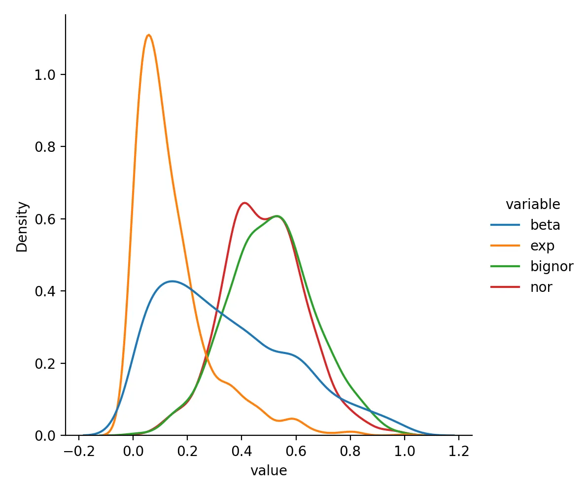
Its biggest advantage is that the output range is fixed and easy to interpret. Its biggest weakness is that strong outliers can squeeze most of the remaining data into a narrow region.

RobustScaler

RobustScaler uses the median and interquartile range, so it is usually more stable when outliers are present.

from sklearn.preprocessing import RobustScaler

df_rsca = pd.DataFrame(RobustScaler().fit(df).transform(df), columns=df.columns)
sns.displot(df_rsca.melt(), x="value", hue="variable", kind="kde")
plt.savefig("robustscaler.png", dpi=200)
plt.close()

Data after RobustScaler transformation looks like this:

beta    exp     bignor  nor
0       0.284395        -0.141315       0.551292        0.923234
1       0.126973        -0.278467       0.779068        0.790394
2       -0.674763       3.388036        0.313090        -1.150118
3       -0.502211       3.251365        1.234674        0.023211
4       0.262573        0.636202        0.729129        0.925553

Distribution is:

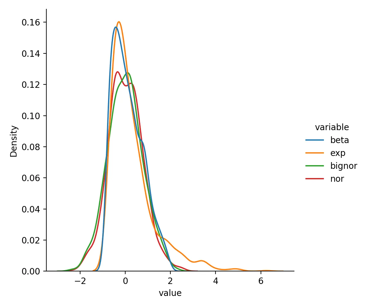
If your data are clearly skewed or contain noticeable outliers, RobustScaler is often a better first check than StandardScaler.

StandardScaler

StandardScaler is the most common standardization method: mean near 0 and standard deviation near 1.

from sklearn.preprocessing import StandardScaler

df_std = pd.DataFrame(StandardScaler().fit(df).transform(df), columns=df.columns)
sns.displot(df_std.melt(), x="value", hue="variable", kind="kde")
plt.savefig("standardscaler.png", dpi=200)
plt.close()

Data after StandardScaler transformation looks like this:

beta    exp     bignor  nor
0       0.252859        -0.460413       0.711804        1.207845
1       0.012554        -0.600899       1.008364        1.030065
2       -1.211305       3.154733        0.401670        -1.566938
3       -0.947902       3.014740        1.601554        0.003337
4       0.219547        0.336005        0.943345        1.210949

Distribution is:

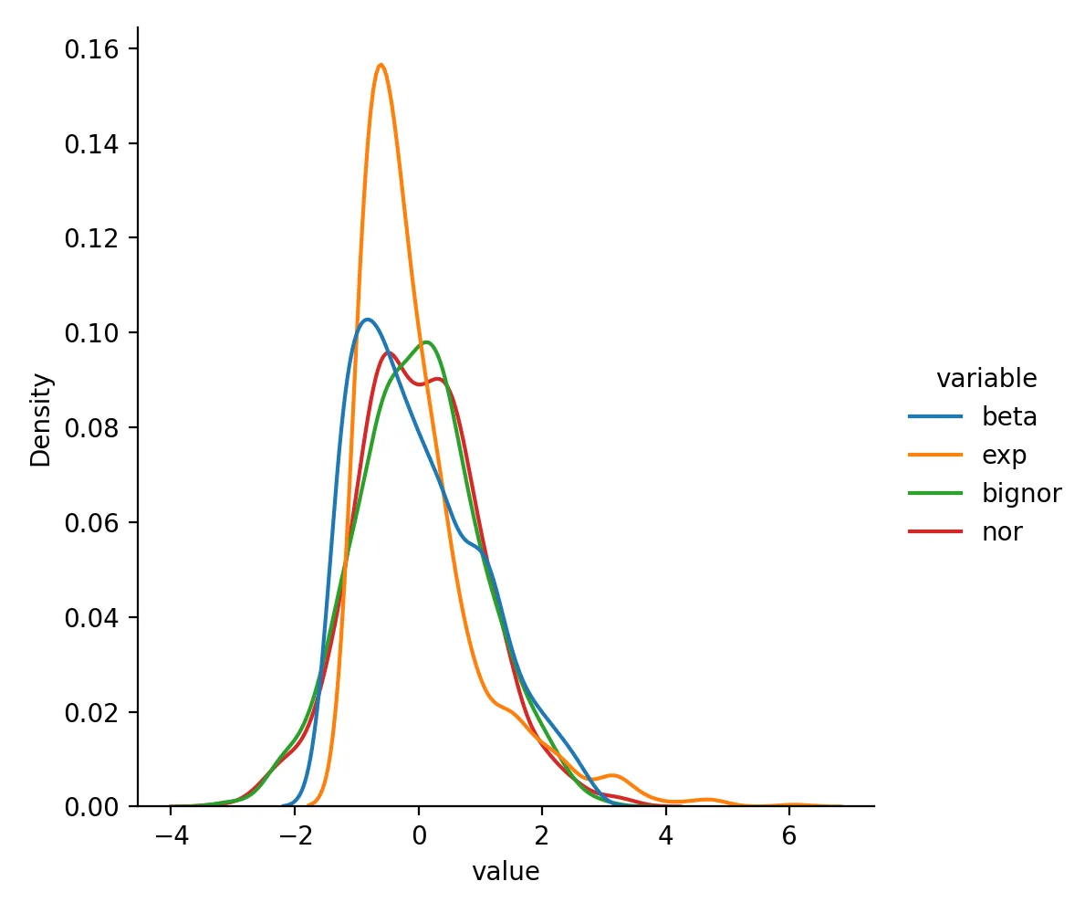
If you do not have a strong reason to choose something else, StandardScaler is often the default starting point for continuous numeric features.

How Normalizer is different

Normalizer is easy to confuse with the three methods above, but its target is different. The three scalers above usually transform each feature column. Normalizer transforms each row so that every sample has unit norm.

A small example:

from sklearn.preprocessing import Normalizer

sample = pd.DataFrame({
    "x1": [3, 1],
    "x2": [4, 2]
})

Normalizer().fit_transform(sample)
# array([[0.6       , 0.8       ],
#        [0.4472136 , 0.89442719]])

This is common in scenarios such as:

1. text vectors
2. sparse features
3. similarity calculations where vector direction matters more than absolute magnitude

So Normalizer is not just another drop-in replacement for StandardScaler or MinMaxScaler.

How to choose in practice

If you want one practical comparison table, use this:

In real work, ask these questions first:

1. Am I scaling features or normalizing whole samples?
2. Are outliers a real issue in this dataset?
3. Does the downstream model care more about distance, gradient behavior, or vector direction?

Summary

This article compared MinMaxScaler, StandardScaler, RobustScaler, and Normalizer, and explained that they solve related but different preprocessing problems.

If you are working with ordinary continuous numeric features, StandardScaler is often the most common starting point. If outliers are obvious, check RobustScaler. If you need a fixed numeric range, use MinMaxScaler. If your real concern is the direction of each sample vector rather than its absolute size, then Normalizer is the one to consider.