Hands-on Implementation of Random Forest Algorithm with Python
Random forest is one of the most common entry points for tabular machine learning because it is relatively stable, works well on structured data, and is easy to get running with sklearn. If you already know the basics of decision trees and supervised learning, this article is enough to start practicing.
This post uses Shanghai weather data to build a small end-to-end regression project whose goal is simple: predict tomorrow’s maximum temperature. The workflow covers environment setup, data loading, cleaning, feature engineering, model training, parameter tuning, and a final single-row prediction example.
The implementation uses Python and sklearn. Docker is only an optional environment choice; if you already have a working local Python data-science setup, you can run the code directly.
Problem Introduction
The problem we want to solve is predicting tomorrow’s maximum temperature in our city using one year’s past weather data. Here I use Shanghai, but you can freely find your city’s data with online climate data tools. We will assume we cannot get the weather forecast and instead make our own predictions through machine learning. What we can get is one year’s historical max temperature, temperatures from the previous two days, and an estimate from a friend who always claims to understand the weather. This is a supervised regression machine learning problem. It is supervised because we have both the features (city data) and the target (temperature) we want to predict. During training, we provide features and targets to the random forest, and it must learn how to map data to predictions. Also, it is a regression task because the target value is continuous (as opposed to discrete classes in classification). That’s almost all the background we need, so let’s get started!
Docker and Jupyter Notebook Setup
Before we start Python programming directly, let’s first establish the required Python environment using Docker:
yum install docker -y  ## Install Docker
docker pull jupyter/datascience-notebook  # Pull machine learning image
mkdir ~/jupyter
cd ~/jupyter
docker run -itd -p 8889:8888 -v jupyter:/home/jovyan jupyter/datascience-notebook  # Run image, map directories
You can check out some basics about Docker in an earlier post.
If you do not want to use Docker, at minimum install these dependencies locally:
pip install pandas numpy scikit-learn matplotlib
Data Collection
First, we need to obtain historical weather data for Shanghai. Weather data in China is mostly paid, so I only could get free data from foreign websites. I used NOAA9 climate data online tool to get Shanghai’s weather data from January 1, 2019, to December 24, 2019. You can place an order by providing your email,
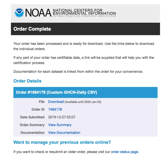
Choose CSV format, then check your email to receive the data,
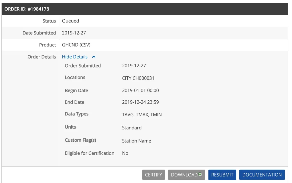
Gmail is recommended. Usually, about 80% of time in data analysis is spent cleaning and retrieving data, but you can reduce this by finding quality data sources. NOAA is the official US weather site providing various weather data. Temperature data is directly downloadable as CSV files, easy to read and parse with Python. The complete data file has been downloaded and placed on this site at:
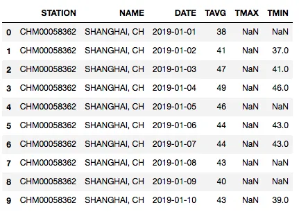
Use pandas to read the data:
# by chunjiangmuke
import pandas as pd

weather = pd.read_csv('1984178.csv')
weather.head(10)
Column descriptions:
- STATION: National city code (this is Shanghai including Hongqiao)
- NAME: City name, Shanghai
- DATE: Date
- TAVG: Average temperature of the day
- TMAX: Max temperature of the day
- TMIN: Min temperature of the day
Detecting Anomalies and Data Transformation
If we look at the data dimensions, we see there are 3605 days’ data. From NOAA data, I found there are two observation areas for Shanghai: Shanghai and Hongqiao. Also, some days are missing, probably not updated yet. This reminds us that real-world data is never perfect. Here, I removed Hongqiao data. Missing or incorrect data or anomalies affect analysis. In this case, missing data has little effect and data quality is generally good due to the source.
# Keep only Shanghai station data
weather = weather[weather.STATION == "CHM00058362"]  # CHM00058362 is Shanghai, CHM00058367 is Hongqiao
import numpy as np
np.shape(weather)

# Output: (3605, 6)
Basic statistics of data:
weather.describe()

# Output example:
# TAVG	TMAX	TMIN
# count	3605.000000	1799.000000	2549.000000
# mean	63.298197	67.204558	57.074147
# std	16.052515	16.498672	16.856828
# min	21.000000	32.000000	18.000000
# 25%	49.000000	53.000000	42.000000
# 50%	65.000000	68.000000	58.000000
# 75%	76.000000	80.000000	72.000000
# max	96.000000	103.000000	89.000000
You can see that some columns contain many missing values, so this example starts with a simple mean-value fill. Because weather has continuity, yesterday’s and the day-before-yesterday’s temperatures are often useful signals, so the code creates lag1 and lag2 features.
One detail matters here: the code below does not actually one-hot encode the month. It keeps month and day as direct numeric features. That is acceptable for a simple teaching example, but if you want a stricter modeling workflow, it is worth comparing against categorical encoding later.
import pandas as pd
import numpy as np
from sklearn.model_selection import train_test_split
from sklearn.ensemble import RandomForestRegressor
from sklearn.metrics import mean_absolute_error

# Read data
weather = pd.read_csv('1984178.csv')

# Keep only Shanghai station data
weather = weather[weather.STATION == "CHM00058362"]

# Fill missing values with column means
weather['TMAX'] = weather['TMAX'].fillna(weather['TMAX'].mean())
weather['TMIN'] = weather['TMIN'].fillna(weather['TMIN'].mean())
weather['TAVG'] = weather['TAVG'].fillna(weather['TAVG'].mean())

# Convert DATE to datetime and extract features
weather['DATE'] = pd.to_datetime(weather['DATE'])
weather['month'] = weather['DATE'].dt.month
weather['day'] = weather['DATE'].dt.day

# Create lag features for previous two days' max temperature
weather['TMAX_lag1'] = weather['TMAX'].shift(1)
weather['TMAX_lag2'] = weather['TMAX'].shift(2)

# Drop rows with NaN values
weather = weather.dropna()

# Define features and target
features = ['month', 'day', 'TMAX_lag1', 'TMAX_lag2', 'TMIN', 'TAVG']
X = weather[features]
y = weather['TMAX']

# Split train and test data
X_train, X_test, y_train, y_test = train_test_split(X, y, test_size=0.2, random_state=42)
Build Random Forest Model
Now we can build and train the random forest model:
from sklearn.ensemble import RandomForestRegressor
from sklearn.metrics import mean_absolute_error

# Initialize random forest regressor
rf = RandomForestRegressor(n_estimators=100, random_state=42)

# Train the model
rf.fit(X_train, y_train)

# Predictions on training set
train_predictions = rf.predict(X_train)

# Predictions on test set
test_predictions = rf.predict(X_test)

# Calculate mean absolute error
train_mae = mean_absolute_error(y_train, train_predictions)
test_mae = mean_absolute_error(y_test, test_predictions)

print(f"Training MAE: {train_mae:.2f}")
print(f"Testing MAE: {test_mae:.2f}")
Model Evaluation and Optimization
Let’s evaluate the model and perform some optimization:
from sklearn.model_selection import GridSearchCV
from sklearn.ensemble import RandomForestRegressor
from sklearn.metrics import mean_absolute_error

# Parameter grid for tuning
param_grid = {
    'n_estimators': [50, 100, 200],
    'max_depth': [None, 10, 20],
    'min_samples_split': [2, 5, 10]
}

# Grid search with 5-fold CV
grid_search = GridSearchCV(estimator=RandomForestRegressor(random_state=42),
                           param_grid=param_grid,
                           cv=5,
                           n_jobs=-1,
                           verbose=2)

grid_search.fit(X_train, y_train)

# Best parameters
print(f"Best parameters: {grid_search.best_params_}")

# Use best estimator for prediction
best_rf = grid_search.best_estimator_
test_predictions = best_rf.predict(X_test)
test_mae = mean_absolute_error(y_test, test_predictions)

print(f"Optimized test MAE: {test_mae:.2f}")
How to tell whether the model is basically usable
For this example, the quickest checks are:
- Compare training MAE and testing MAE to see whether overfitting is obvious
- Run one single-row prediction to confirm the input schema and prediction path are both correct
If training error is much lower than test error, the model is usually memorizing the training data too aggressively and needs further tuning.
Complete Prediction Workflow
Finally, we can use the trained model to make actual predictions:
def predict_temperature(model, last_two_days):
    """
    Predict tomorrow's max temperature

    Parameters:
    model -- trained random forest model
    last_two_days -- DataFrame containing weather data for the last two days

    Returns:
    Predicted max temperature for tomorrow
    """
    features = ['month', 'day', 'TMAX_lag1', 'TMAX_lag2', 'TMIN', 'TAVG']

    if not all(f in last_two_days.columns for f in features):
        raise ValueError("Input data is missing required features")

    prediction = model.predict(last_two_days[features])

    return prediction[0]

# Example usage
sample_data = pd.DataFrame({
    'month': [12],
    'day': [25],
    'TMAX_lag1': [50],  # Yesterday's max temp
    'TMAX_lag2': [48],  # Day before yesterday's max temp
    'TMIN': [40],       # Today's min temp
    'TAVG': [45]        # Today's avg temp
})

predicted_temp = predict_temperature(best_rf, sample_data)
print(f"Predicted max temperature for tomorrow: {predicted_temp:.1f}°F")
Summary
In this article, we completed the following:
- Obtained and cleaned Shanghai weather data from NOAA
- Performed feature engineering by creating lag features
- Built and trained a random forest regression model
- Optimized model parameters using grid search
- Analyzed feature importance
- Created a complete prediction workflow
This model can predict Shanghai’s maximum temperature quite accurately, with mean absolute error around 2-3°F. To further improve performance, consider:
- Adding more historical weather data
- Introducing other meteorological features like humidity, precipitation, etc.
- Trying other machine learning algorithms for comparison
- Using more complex time series processing methods
Related reading
- 原文作者:春江暮客
- 原文链接:https://www.bobobk.com/en/621.html
- 版权声明:本作品采用 知识共享署名-非商业性使用-禁止演绎 4.0 国际许可协议 进行许可,非商业转载请注明出处(作者,原文链接),商业转载请联系作者获得授权。