Application of Python Implementation of Gradient Descent in Practice
Definition
Gradient descent is a first-order optimization algorithm, commonly called the steepest descent method. To find a local minimum of a function using gradient descent, one must iteratively move from the current point in the opposite direction of the gradient (or approximate gradient) by a specified step size. Conversely, if the search moves iteratively in the direction of the gradient, it approaches a local maximum of the function; this process is called gradient ascent.
If you are new to machine learning, the easiest intuition is this:
“Stand on a hill, take a small step in the steepest downhill direction, and repeat until you get close to the bottom.”
This article uses the simplest quadratic example to make that process concrete.
Example Demonstration and Explanation of Gradient Descent Algorithm
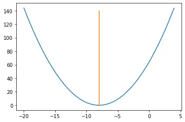
Gradient descent is generally used in loss functions. Suppose ( y = (x + 8)^2 ) is a loss function.
import matplotlib.pyplot as plt
import numpy as np
x = np.arange(-20, 4, 0.01)
y = (x + 8)*(x + 8)
plt.plot(x,y)
plt.plot([-8,-8],[0,140])
Solution: Just by looking at the chart, we know the answer. When ( x = -8 ) (i.e., ( x = -8, y = 0 )), ( y = (x + 8)^2 ) reaches its minimum. Therefore, ( x = -8 ) is the local and global minimum of the function.
Now, let’s see how to use gradient descent to obtain the same value.
Step 1: Initialize ( x = -3 ). Then find the gradient of the function ( frac{dy}{dx} = 2(x + 8) ).
Step 2: Move in the negative direction of the gradient (why?). But how much to move exactly? For this, we introduce the learning rate, which adjusts the step size in the direction of the gradient. Here, assume learning rate → 0.01.
Step 3: Let’s perform two iterations of gradient descent:
# Initialize x0 = -3, rate = 0.01, dy/dx = 2(x + 8)

# First iteration
# x1 = x0 - rate*(dy/dx) = -3 - 0.01*(2*(-3 + 8)) = -3.1
# Second iteration
# x2 = x1 - rate*(dy/dx) = -3.1 - 0.01*(2*(-3.1 + 8)) = -3.198
Step 4: We observe that the X value is slowly decreasing and should eventually converge to -8 (the local minimum). But how many iterations should we perform?
Because the algorithm can infinitely approach -8 but cannot run forever, we set a precision variable in the algorithm that calculates the difference between two consecutive ( x ) values, i.e., the change in ( x ). If the difference between two consecutive iterations of ( x ) is less than our set precision, we stop the computation and obtain the result.
The three most important parameters in this example
In practice, gradient descent behavior is mostly controlled by these three quantities:
initx— the starting pointrate— the learning rate, which controls how far each step movescutoff— the stopping precision
If the learning rate is too large, the updates can overshoot the optimum or oscillate. If it is too small, convergence becomes unnecessarily slow.
Gradient Descent in Python
Here, we use Python gradient descent to find the minimum of the function ( y = (x + 8)^2 ).
Step 1: Initialize values
initx = -3  # algorithm starts at x = -3
rate = 0.01  # learning rate
cutoff = 0.000001  # precision, tells when to stop the algorithm
previous_step_size = 1  #
max_iters = 100000  # maximum iterations
iters = 0  # iteration counter
df = lambda x: 2 * (x + 8)  # slope of our function, gradient direction
f = lambda x: (x + 8) * (x + 8)  # objective function
Step 2: Loop and find the minimum
while previous_step_size > cutoff and iters < max_iters:
    prev_x = initx  # Store current x value in prev_x
    initx -= rate * df(prev_x)  # Gradient descent step
    previous_step_size = abs(initx - prev_x)  # Change in x
    iters = iters + 1  # iteration count
    print("Iteration", iters, "\nX value:", initx, "\nCurrent f(x):", f(initx))

print("Minimum found at:", initx)
Result:
Iteration 1
X value: -3.1
Iteration 2
X value: -3.198
Iteration 3
X value: -3.29404
Iteration 4
X value: -3.3881592
Iteration 5
X value: -3.480396016
···
Iteration 186
X value: -7.883313642475223
Iteration 187
X value: -7.885647369625718
Iteration 188
X value: -7.8879344222332035
Iteration 189
X value: -7.890175733788539
Iteration 190
X value: -7.892372219112769
Iteration 191
X value: -7.894524774730513
Iteration 192
X value: -7.8966342792359026
Iteration 193
X value: -7.898701593651184
Iteration 194
X value: -7.900727561778161
····
Iteration 565
X value: -7.999944830027104
Iteration 566
X value: -7.999945933426562
Iteration 567
X value: -7.999947014758031
Iteration 568
X value: -7.99994807446287
Iteration 569
X value: -7.999949112973613
Iteration 570
X value: -7.99995013071414
Iteration 571
X value: -7.999951128099857
Minimum found at -7.999951128099857
From the results, by iteration 194 the value reached approximately -7.9, and by iteration 571 it reached the target precision. The accuracy improves rapidly in the early iterations and slows down in later stages.
How to check whether your gradient descent loop is behaving correctly
At minimum, verify these three points:
- The function value is generally decreasing over iterations
xis moving toward the theoretical optimum-8- Changing the learning rate affects convergence speed in the expected way
For example, try making rate larger or smaller and compare both the iteration count and the final result. That is the fastest way to build intuition for learning-rate tuning.
Conclusion
This article walked through finding the minimum of a quadratic function step-by-step and explored how to use iteration to find the minimum. This is also the basis of the backpropagation algorithm in neural networks. Mastering it well is helpful to understand neural networks better.
Related reading
- 原文作者:春江暮客
- 原文链接:https://www.bobobk.com/en/648.html
- 版权声明:本作品采用 知识共享署名-非商业性使用-禁止演绎 4.0 国际许可协议 进行许可,非商业转载请注明出处(作者,原文链接),商业转载请联系作者获得授权。