Statistical Skew Distributions Reveal Statistical Traps in Life

When people hear statements like “90% of drivers think they are above average,” the first reaction is often that everyone is overestimating themselves. Statistically, though, that conclusion is not always justified.

The real question is: what does “average” mean here? If the distribution is strongly skewed, the mean and the median can be far apart, and the phrase “above average” can become misleading even when the data itself is real.

This article uses a simple example to show why the mean can be deceptive in skewed data and why the median is often a better reference for what people intuitively think of as a “normal level.”

Let’s look at a practical example to show the unreliability of the mean. Suppose

import numpy as np
import matplotlib.pyplot as plt

a = np.array([1.0,8.6,8.4,8.7,8.8,8.9,8.9,9.0,9.1])

print(a.mean())
print(np.median(a))

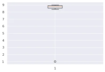
plt.boxplot(a)
# 7.933333333333334
# 8.8

The result looks like this:

Because of one outlier, the mean changes significantly, causing other values to be greater than the mean. The difference lies in whether we use the mean or the median to represent the “average” driver skill level. Using the mean, we add all values and divide by the number of values, resulting in a dataset mean of 7.9. Since 9 out of 10 drivers scored higher than this, 90% of drivers can be considered above average!

On the other hand, the median is found by sorting values from lowest to highest and choosing the middle value where half the data points are smaller and half are larger. This is 8.8, with 5 drivers below and 5 drivers above. By definition, 50% of drivers are below the median, and 50% are above it. If the question is, “Do you think you are better than 50% of other drivers?” then more than 90% of drivers cannot answer truthfully.

(The median is a special case of a percentile (also called quantile), which is the value below which a given percentage of data falls. The median is the 50th percentile: 50% of the data is below this number. We can also find the 90th percentile, where 90% of the values are smaller; and the 10th percentile, where 10% are smaller. Percentiles provide an intuitive way to describe data.)

One practical rule to remember first

If the data contains obvious outliers or the distribution is strongly skewed, do not jump to the mean first.

A safer order is usually:

1. Look at the shape of the distribution
2. Check the median
3. Then decide whether the mean is still informative enough to report

Why is this important

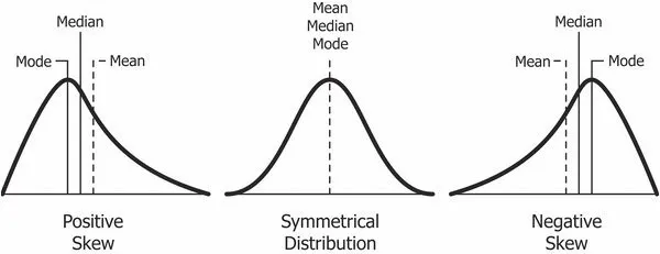
This may seem like a contrived example or a technical issue, but in the real world, it is common for mean and median to disagree. When values are symmetrically distributed, the mean equals the median. However, real-world datasets almost always have some skew, whether positive (right skew) or negative (left skew):

In a positively skewed distribution, the mean is greater than the median. This happens when there are relatively few outliers on the high end, causing a right “skew,” while most values cluster at the lower end. A real-world example is personal income, where the average income is much higher than the median income. The figure below shows a histogram percentile of US income distribution in 2017.

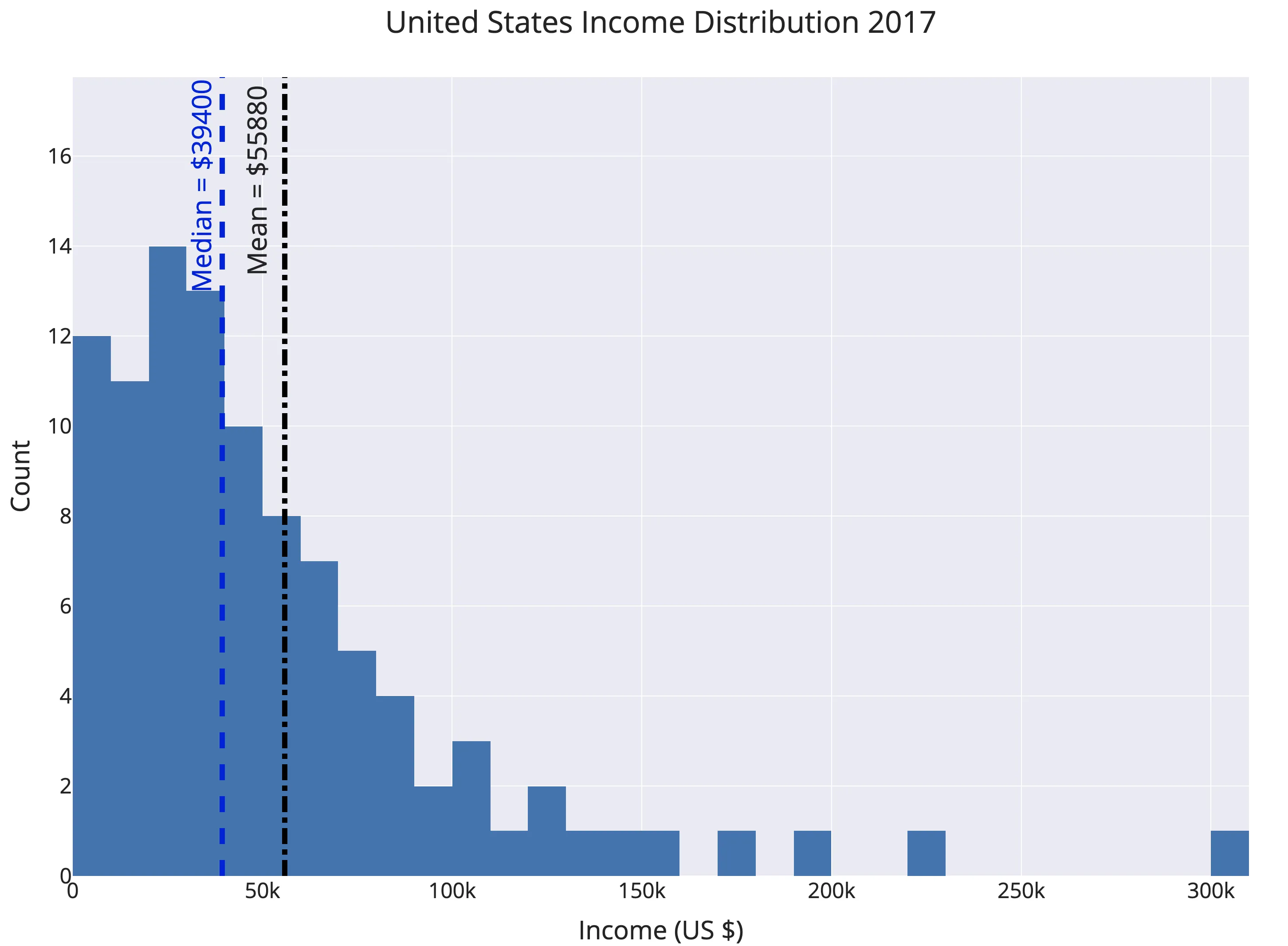
The overall pattern is clear: some very high incomes skew the chart right (positive), making the mean higher than the median. The value $55,880 represents the median, while the mean is closer to the 66th percentile. The explanation is that 66% of Americans earn less than the average national income — when the average is the mean! This phenomenon happens in almost every country.

An example of left skew is age at death. Unfortunately, in this dataset, some deaths occur at relatively young ages, lowering the mean and skewing the chart left (negative skew).

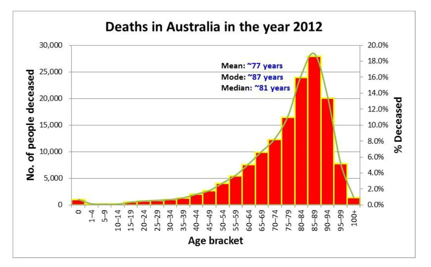
In a negatively skewed case, the median is greater than the mean. The result is that when the mean is defined as the average, more people can be above “average.” The headline “Most people live longer than the average lifespan” may seem strange, but if you carefully select the statistics, you can find this.

Most datasets involving human behavior show some bias. As the saying goes, “Heaven’s way takes away the excess and makes up for the deficiency; Man’s way takes away the deficiency to serve the excess.” Stock market returns, incomes, social media followers, wartime deaths, and city sizes all exhibit highly skewed distributions, many of which fit this pattern. Humans evolved in relatively equal and harmonious conditions, where datasets were normally distributed, but modern life is dominated by unequal distributions. Living in extremes provides incredible reward opportunities, but those rewards go to very few. This also means we must be cautious when discussing mean and median as “average” representations of datasets.

How to avoid being misled in practical analysis

If you are looking at income, followers, city size, click volume, or similar data, it is worth doing at least these checks:

1. Plot a boxplot or histogram
2. Report both the mean and the median
3. Inspect whether a small number of outliers is dominating the result

In many cases, the most useful explanation is not just “what is the average,” but “what does the full distribution actually look like?”

Conclusion

In statistics, always remind yourself that when you specify “average,” you need to clarify if you mean the mean or the median, as they differ. The world is not symmetrically distributed, so we should not expect the mean and median of a distribution to be the same.

Machine learning may attract everyone’s attention, but the truly important part of data science is the part we use every day: basic statistics help us understand the world. Being able to distinguish the difference between mean and median may seem ordinary and simple, but compared to knowing how to build neural networks, it is truly relevant to our daily lives. Don’t be misled by appearances — learn to see the essence behind phenomena.

Related reading

• Application of Python Implementation of Gradient Descent in Practice