Bayesian Theory and Practical Python Applications
Bayesian theory provides a principled method for calculating conditional probabilities. With it, we can easily compute conditional probabilities for events where intuition often fails.
Bayesian theory is not only a powerful tool in the field of probability, but also widely used in machine learning. It is used to fit probabilistic models to training datasets (called Maximum A Posteriori or MAP), and in developing models for classification problems such as the Bayesian optimal classifier and Naive Bayes. In this article, you’ll discover Bayes’ Theorem for computing conditional probability and how it is used in machine learning. Before reading this article, it’s recommended to first learn about confusion matrices in machine learning.
This article will cover:
- Bayes’ Theorem for conditional probability
- Explanation of common terminology
- Example calculations using Bayes’ Theorem
- Diagnostic testing scenario
- Manual calculation
- Python computation
1. Bayes’ Theorem for Conditional Probability
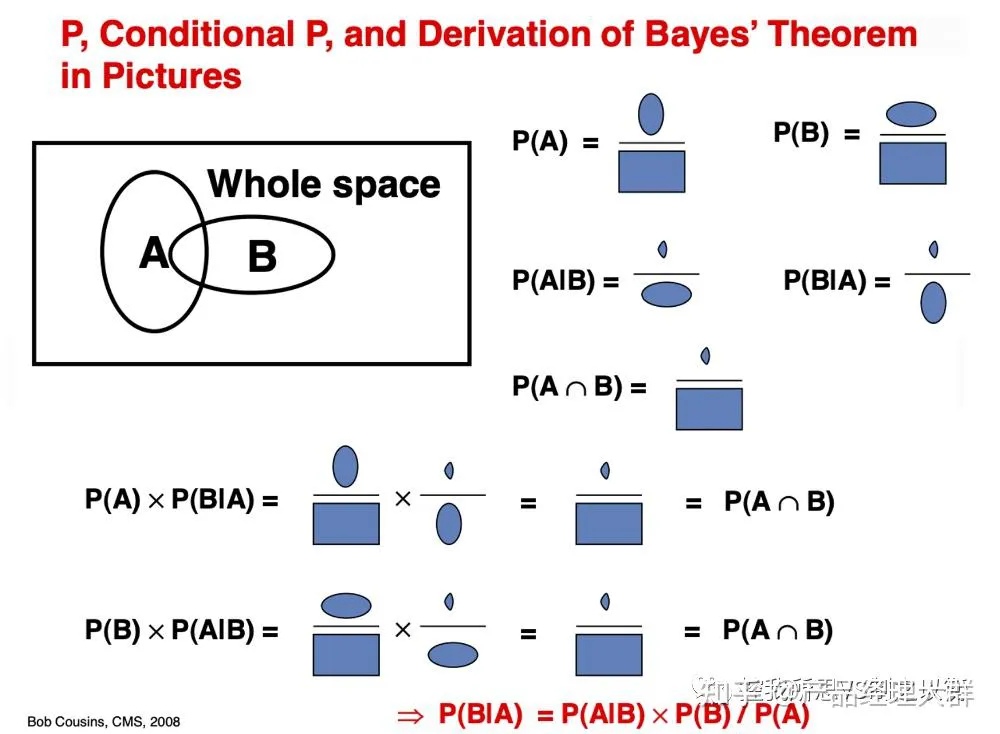
Before diving into Bayes’ Theorem, let’s review marginal, joint, and conditional probabilities.
1.1 General Conditional Probability
Marginal probability is the probability of an event, irrespective of other variables. If the variables are independent, this is simply the event’s probability; otherwise, it’s the sum of probabilities across all possible outcomes of the other variables (called the sum rule).
- Marginal probability: the probability of an event, such as P(A), regardless of other variables.
Joint probability is the probability of two (or more) events occurring together, such as the probability of events A and B (e.g., variables X and Y). It’s usually written as A and B.
- Joint probability: the probability of two (or more) events occurring simultaneously, such as P(A and B) or P(A, B).
Conditional probability is the probability of one event occurring given that another has occurred. It’s written as P(A | B), the probability of A given B.
- Conditional probability: the probability of one (or more) events given another, such as P(A | B).
You can compute joint probability using conditional probability, for example:
- P(A, B) = P(A | B) * P(B)
This is called the product rule. Importantly, joint probability is symmetric:
- P(A, B) = P(B, A)
Conditional probability can also be computed using joint probability:
- P(A | B) = P(A, B) / P(B)
However, conditional probability is not symmetric:
- P(A | B) != P(B | A)
1.2 Bayes’ Theorem for Conditional Probability
Bayes’ Theorem allows us to compute one conditional probability from another:
- P(A | B) = P(B | A) * P(A) / P(B)
- Similarly, P(B | A) = P(A | B) * P(B) / P(A)
This alternative method is useful when joint probability is hard to compute, or when the reverse conditional probability is available.
This form of conditional probability calculation is called Bayes’ Rule or Bayes’ Theorem, named after Reverend Thomas Bayes.
Bayes’ Theorem: A principle for calculating conditional probability without joint probability.
We often can’t directly compute the denominator (P(B)), but we can use:
- P(B) = P(B | A) * P(A) + P(B | not A) * P(not A)
So the full formula becomes:
- P(A | B) = P(B | A) * P(A) / [P(B | A) * P(A) + P(B | not A) * P(not A)]
Note: the denominator is just the expansion using the law of total probability.
For example:
- P(not A) = 1 – P(A)
- P(B | not A) = 1 – P(not B | not A)
Now that we’re familiar with the computation, let’s break down the terms in the equation.
2. Explanation of Common Terms
The terms in Bayes’ Theorem vary depending on context.
Typically, the result P(A | B) is called the posterior, and P(A) is called the prior.
- P(A | B): posterior probability
- P(A): prior probability
P(B | A) is called the likelihood, and P(B) is the evidence.
- P(B | A): likelihood
- P(B): evidence
Thus, Bayes’ Theorem can be rewritten as:
Posterior = Likelihood * Prior / Evidence
Let’s clarify this with a smoking and cancer example:
Suppose a person smokes. What is the probability they have cancer?
- P(Cancer | Smoking) = P(Smoking | Cancer) * P(Cancer) / P(Smoking)
With this understanding, let’s look at a practical scenario.
3. Bayes’ Theorem Example Calculation
To understand Bayes’ Theorem, we use a medical example involving a diagnostic test.
3.1 Diagnostic Testing Scenario
Medical tests are not perfect. For example, consider a COVID-19 test kit with 99% sensitivity, 98% specificity, and a 0.0001 (0.01%) infection rate in the general population. If someone tests positive, what’s the probability they actually have COVID-19?
3.2 Manual Probability Calculation
Let’s start with sensitivity: the proportion of true positives.
- P(Test = Positive | COVID = True) = 0.99
Intuitively, we may think a positive test means a 99% chance of infection, but that’s wrong.
This is called the base rate fallacy—ignoring the low infection rate in the population.
Base rate:
- P(COVID = True) = 0.0001 (0.01%)
We calculate:
- P(COVID = True | Test = Positive) = (0.99 * 0.0001) / P(Test = Positive)
Now compute P(Test = Positive):
- P(Test = Positive) = P(Test = Positive | COVID = True) * P(COVID = True) + P(Test = Positive | COVID = False) * P(COVID = False)
First, compute:
- P(COVID = False) = 1 – 0.0001 = 0.9999
Assume specificity = 98%, so:
- P(Test = Negative | COVID = False) = 0.98
- P(Test = Positive | COVID = False) = 1 – 0.98 = 0.02
Then:
- P(Test = Positive) = 0.99 * 0.0001 + 0.02 * 0.9999 = 0.000099 + 0.019998 = 0.020097
Finally:
- P(COVID = True | Test = Positive) = 0.000099 / 0.020097 ≈ 0.00493
So, despite testing positive, there’s only a 0.493% chance the person actually has COVID-19!
This surprising result highlights how real probabilities can defy our intuition.
To use Bayes’ Theorem, we need:
- Base rate (prior)
- Sensitivity (true positive rate)
- Specificity (true negative rate)
Even without P(Test = Positive), we can compute it from the above.
With more context (e.g., age, location), Bayes’ Theorem can give even more accurate estimates.
Python Computation
Here’s a Python implementation of the scenario:
# Given P(A), P(B|A), P(B|not A), compute P(A|B)
def bayes_theorem(p_a, p_b_given_a, p_b_given_not_a):
    # calculate P(not A)
    not_a = 1 - p_a
    # calculate P(B)
    p_b = p_b_given_a * p_a + p_b_given_not_a * not_a
    # calculate P(A|B)
    p_a_given_b = (p_b_given_a * p_a) / p_b
    return p_a_given_b

# P(A)
p_a = 0.0001
# P(B|A)
p_b_given_a = 0.99
# P(B|not A)
p_b_given_not_a = 0.02
# Compute P(A|B)
result = bayes_theorem(p_a, p_b_given_a, p_b_given_not_a)
# Print result
print('P(A|B) = %.3f%%' % (result * 100))
# P(A|B) = 0.493%
Summary
This article started with conditional probability, introduced Bayes’ Theorem, and showed how it corrects our misleading intuition. In the example, even with 99% sensitivity and 98% specificity, and a base rate of 0.01%, a positive test still only yields a 0.493% chance of actual infection.
This demonstrates the importance of using a scientific approach over intuition when interpreting probabilities.
- 原文作者:春江暮客
- 原文链接:https://www.bobobk.com/en/823.html
- 版权声明:本作品采用 知识共享署名-非商业性使用-禁止演绎 4.0 国际许可协议 进行许可,非商业转载请注明出处(作者,原文链接),商业转载请联系作者获得授权。