SomaticSignatures Tutorial: Analyze Tumor Mutation Signatures from TCGA Data

SomaticSignatures is an R package for analyzing tumor single-nucleotide variant patterns. A common use case is extracting potential mutational signatures from sequence-context data to help interpret tumor development and evolution.

This post keeps the theory light and focuses on a workflow you can reuse directly: clean TCGA MAF data into the format expected by SomaticSignatures, then use R to estimate the number of signatures, run NMF decomposition, and visualize the results.

Before you start

Before running the workflow, check these three points first:

1. You already have a mutation table containing SNP records
2. The reference genome version matches the BSgenome package used in the analysis, here hg38
3. The sample count is not too small, otherwise the decomposition can become unstable

Data Preparation

SomaticSignatures does not need many columns, but you should at least reshape the input into these fields:

• Sample
• chr
• start
• ref
• alt

If you downloaded a raw TCGA MAF file, a small Python preprocessing step is usually the quickest way to keep only SNP records and rename the fields into something the R code can consume directly.

Example preprocessing script:

import pandas as pd

df = pd.read_csv("TCGA.CRC.mutect.maf.csv")
df.head()
"""
  Hugo_Symbol  Entrez_Gene_Id  ... MC3_Overlap GDC_Validation_Status
0      UBE2J2          118424  ...        True               Unknown
1       RPL22            6146  ...        True               Unknown
2     TNFRSF9            3604  ...        True               Unknown
3     EXOSC10            5394  ...       False               Unknown
4      PTCHD2           57540  ...        True               Unknown
"""
df = df[df.Variant_Type=='SNP']
# First filter SNP data
newdf = df.iloc[:,[33,4,5,11,12]]
# Select specific columns
newdf.columns = ["Sample","chr", "start","ref",  "alt"]
newdf.ref = newdf.ref.str[:1]
# Remove rows where ref and alt are the same to avoid errors later
newdf = newdf[newdf.ref != newdf.alt]
# Save data for R analysis
newdf.to_csv("TCGA.CRC.mutect.maf.filtered.csv",index=None)

The goal of this step is simple: reduce a large, noisy MAF table into a clean SNP table for downstream R analysis.

Signature Selection

The downstream analysis is done in R because signature extraction and plotting are handled by the SomaticSignatures ecosystem.

First install the required packages:

install.packages(c("SomaticSignatures","SomaticCancerAlterations","BSgenome.Hsapiens.UCSC.hg38","data.table"))

Load the libraries:

suppressPackageStartupMessages(library(SomaticSignatures))
suppressPackageStartupMessages(library(SomaticCancerAlterations))
suppressPackageStartupMessages(library(BSgenome.Hsapiens.UCSC.hg38))
suppressPackageStartupMessages(library(data.table))
suppressPackageStartupMessages(library(ggplot2))

Then read the cleaned table and convert it into VRanges, which mutationContext expects:

df=fread('TCGA.CRC.mutect.maf.filtered.csv',data.table = F)
# ["Sample","chr", "start","end","ref",  "alt"]
alls=as.character(unique(df$Sample))
df$study=df$Sample

sca_vr = VRanges(
  seqnames =  df$chr ,
  ranges = IRanges(start = df$start,end = df$start+1),
  ref = df$ref,
  alt = df$alt,
  sampleNames = as.character(df$Sample),
  study=as.character(df$study))

Next, build the mutation-context matrix and evaluate how many signatures may be appropriate:

sca_motifs = mutationContext(sca_vr, BSgenome.Hsapiens.UCSC.hg38)
head(sca_motifs)
# For each sample, calculate the proportion distribution of 96 mutation possibilities
escc_sca_mm = motifMatrix(sca_motifs, group = "study", normalize = TRUE)
dim( escc_sca_mm )
table(colSums(escc_sca_mm))
head(escc_sca_mm[,1:4])
n_sigs = 5:15
gof_nmf = assessNumberSignatures(escc_sca_mm , n_sigs, nReplicates = 5)
save(gof_nmf,file = 'gof_nmf.Rdata')
load(file = 'gof_nmf.Rdata')
# This assessNumberSignatures step is very time-consuming.
pdf("plotNumberSignatures.pdf",width=18, height=7)
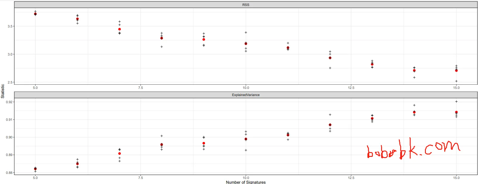
plotNumberSignatures(gof_nmf)
dev.off()

The most time-consuming step is usually:

assessNumberSignatures(escc_sca_mm , n_sigs, nReplicates = 5)

If you increase the number of samples or the number of replicates, runtime rises quickly.

Example result:

From this plot, the explained variance is already close to 99% when the number of signatures reaches around 13, so additional signatures may bring diminishing returns.

Signature Plotting

Once you decide on a reasonable signature count, you can run the decomposition and generate the plots. The original example uses 11, but in practice you should compare that choice against the previous trend plot.

sigs_nmf = identifySignatures(escc_sca_mm  ,
                             11, nmfDecomposition)
save(escc_sca_mm,sigs_nmf,file = 'escc_denovo_results.Rata')

load(file = 'escc_denovo_results.Rata')
str(sigs_nmf)
library(ggplot2)
pdf("maf.pdf",width=18, height=7)
plotSignatureMap(sigs_nmf) + ggtitle("Somatic Signatures: NMF - Heatmap")
plotSignatures(sigs_nmf, normalize =T) +
  ggtitle("Somatic Signatures: NMF - Barchart")  +
  facet_grid(signature ~ alteration,scales = "free_y")
dev.off()

Example output:

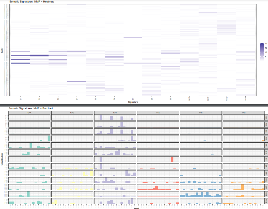
In practice, you usually look at two plot types here:

1. plotSignatureMap heatmaps for the overall distribution of signatures across samples
2. plotSignatures bar charts for the substitution pattern inside each signature

How to sanity-check the result

Generating a plot does not automatically mean the decomposition is reliable. At minimum, check these points:

1. Whether the explained variance curve is already flattening out
2. Whether each signature still shows an interpretable biological pattern instead of obvious noise
3. Whether the result remains roughly stable after small parameter changes or sample changes

If you later want to compare your de novo signatures with known COSMIC signatures, this step works well as the initial exploration stage.

How SomaticSignatures compares with newer tools

If you are starting mutational signature analysis today, you will usually also run into MutationalPatterns and SigProfiler.

A practical summary is:

1. SomaticSignatures is straightforward for learning the 96-context workflow, NMF decomposition, and the core plotting steps
2. MutationalPatterns is more active within the Bioconductor ecosystem and is often more convenient for extended analysis and comparisons with known signatures
3. SigProfiler is commonly used for signature extraction and COSMIC-oriented workflows, and appears more often in newer papers

If your goal is to understand the underlying workflow and build a small interpretable R pipeline, SomaticSignatures is still useful. If you need a more complete modern workflow for fitting, exposure analysis, or alignment with recent publications, it is worth looking at MutationalPatterns or SigProfiler next.

Common issues

1. mutationContext fails with a reference-genome-related error

First check whether the chromosome naming style and the reference genome version are consistent, for example hg38 with chromosome names like chr1.

2. Why remove rows where ref and alt are the same?

Because those records do not represent real substitutions and usually only add noise or trigger downstream errors.

3. Why choose 11 signatures or 13 signatures?

There is no fixed answer. The correct choice should come from the plotNumberSignatures trend, especially around the plateau region, instead of copying a single number mechanically.

Summary

This article shows a practical workflow: use Python to clean TCGA SNP data, then use SomaticSignatures to build the 96-context mutation matrix, estimate signature counts, and plot NMF-based de novo signatures.

The real value of this approach is not reproducing one fixed number, but exploring signatures directly from your own cohort first and only then deciding whether to compare them with COSMIC or another known signature catalog. For tumor-specific studies, that is often the more useful path.