Calculating Confidence Intervals with Bootstrapping: A Python Resampling Example

A confidence interval (CI) is used to express the uncertainty around an estimate. In practice, the 95% confidence interval is the form people see most often in data analysis and scientific writing.

This article keeps the theory brief and focuses on a practical example: how to use Python bootstrapping to repeatedly resample a dataset and estimate the 95% confidence interval of the sample mean.

Concept

A useful interpretation is this: a confidence interval does not mean there is a 95% probability that the true parameter is inside one specific interval. It means that if you repeated the full sampling-and-interval process many times, about 95% of those intervals would contain the true parameter.

Why Use Confidence Intervals

In real work, we usually observe a sample rather than the full population. A single mean or proportion does not express uncertainty very well, so confidence intervals help by describing both the estimate and the range of plausible variation around it.

Calculation of Confidence Interval

If the data are approximately normal and you are using the classical parametric approach, common confidence levels correspond to these z-scores:

Confidence Interval  z-score
0.90                1.645
0.95                1.96
0.99                2.58

The classical formula is:

That is, you take the sample mean and add or subtract the error term to obtain the lower and upper bounds.

But many real datasets do not fit the assumptions of the parametric formula very cleanly. That is where bootstrap methods become useful.

How bootstrapping works

The core bootstrap idea is straightforward:

1. Resample from the observed data with replacement
2. Build a new sample each time
3. Compute the statistic you care about, such as the mean or median
4. Repeat this many times to form an empirical distribution of that statistic
5. Use percentiles of that empirical distribution to estimate a confidence interval

Application

Now for the practical part. Below is a simple example showing how to estimate a 95% bootstrap confidence interval for the sample mean.

First, Generating the Data

import numpy as np
import pandas as pd
import matplotlib.pyplot as plt
import seaborn as sns
np.random.seed(1024)
data_nor = np.random.normal(loc=1, scale=2, size=1000)

This gives us a simulated sample with mean around 1 and standard deviation around 2.

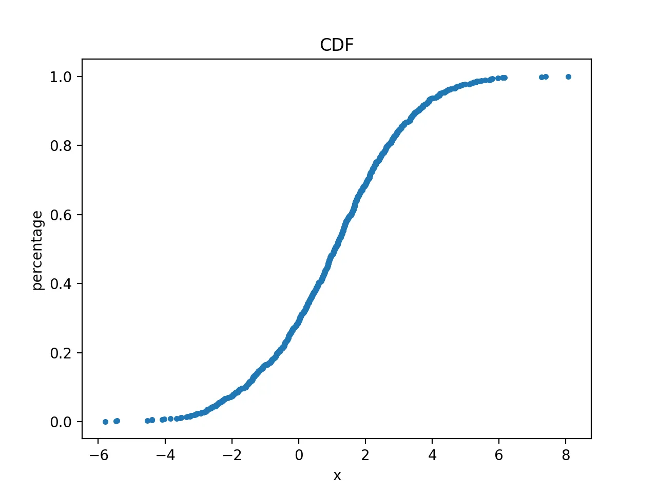
Viewing Its Cumulative Distribution Curve

First, plot the empirical cumulative distribution function (CDF):

x = np.sort(data_nor)
n = len(x)
y = np.arange(1, n+1) / n
plt.plot(x, y, marker='.', linestyle="none")
plt.xlabel("x")
plt.ylabel("percentage")
plt.title("CDF")
plt.savefig("cdf.png", dpi=200)
plt.close()

The resulting plot is:

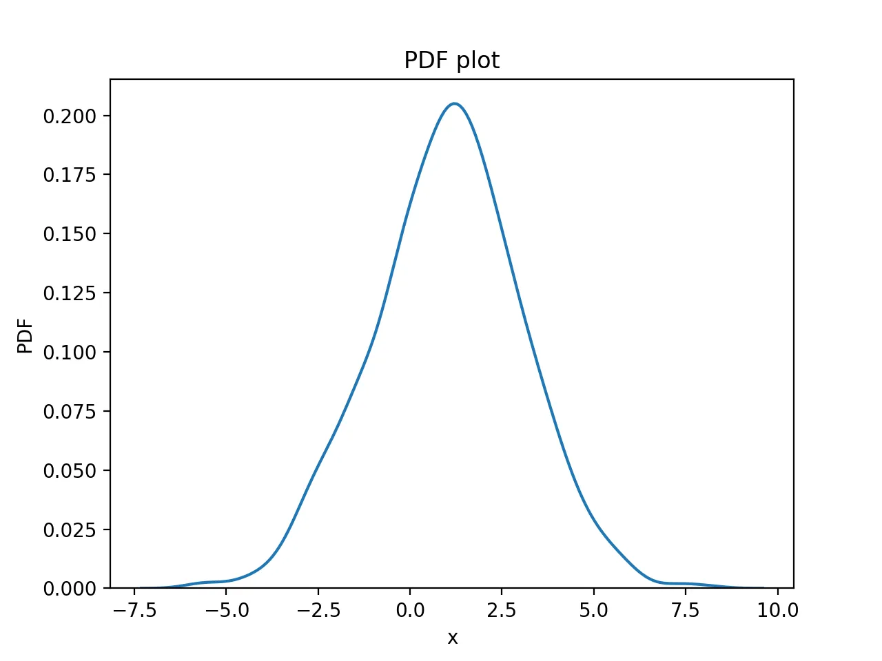
Viewing Its Density Curve

Then inspect the density curve:

sns.kdeplot(data_nor, fill=False)
plt.xlabel("x")
plt.ylabel("PDF")
plt.title("PDF plot")
plt.savefig("pdf.png", dpi=200)
plt.close()

The plot is:

Generating Background Data Randomly via Bootstrapping and Calculating Confidence Interval

By repeatedly sampling from data_nor with replacement, we can build a bootstrap distribution of the sample mean. One important detail matters here:

• if the goal is a confidence interval for the mean, the percentile calculation must be applied to bs_mean
• not to the last raw bs_sample

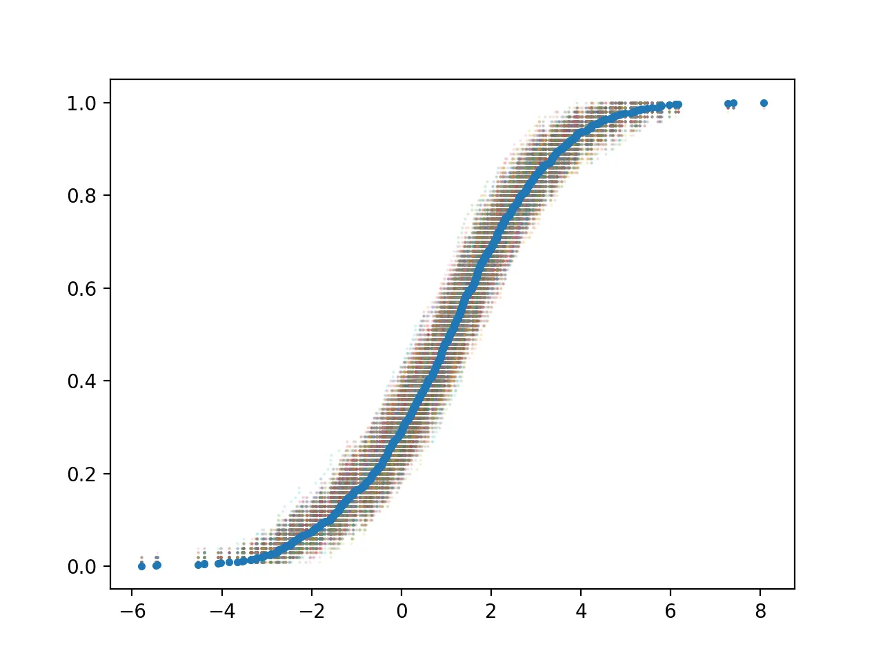
# First plot the original data as the middle curve
plt.plot(x, y, marker='.', linestyle="none")
bs_mean = []
for i in range(10000):
    bs_sample = np.random.choice(data_nor, size=100, replace=True)
    x_bs = np.sort(bs_sample)
    bs_mean.append(np.mean(bs_sample))
    n_bs = len(x_bs)
    y_bs = np.arange(1, n_bs+1) / n_bs
    plt.scatter(x_bs, y_bs, s=1, marker='.', alpha=0.02)
plt.savefig("bs.png", dpi=200)
plt.close()

The resulting plot is:

Next, plot the distribution of bs_mean and mark the 2.5% and 97.5% percentile bounds:

ci_low, ci_high = np.percentile(bs_mean, [2.5, 97.5])

plt.hist(bs_mean, bins=50, density=True)
plt.axvline(x=ci_low, ymin=0, ymax=1, label='2.5%', c='y')
plt.axvline(x=ci_high, ymin=0, ymax=1, label='97.5%', c='r')
plt.xlabel("x")
plt.ylabel("PDF")
plt.title("BS PDF")
plt.legend()
plt.savefig("percent.png", dpi=200)
plt.close()

The plot is:

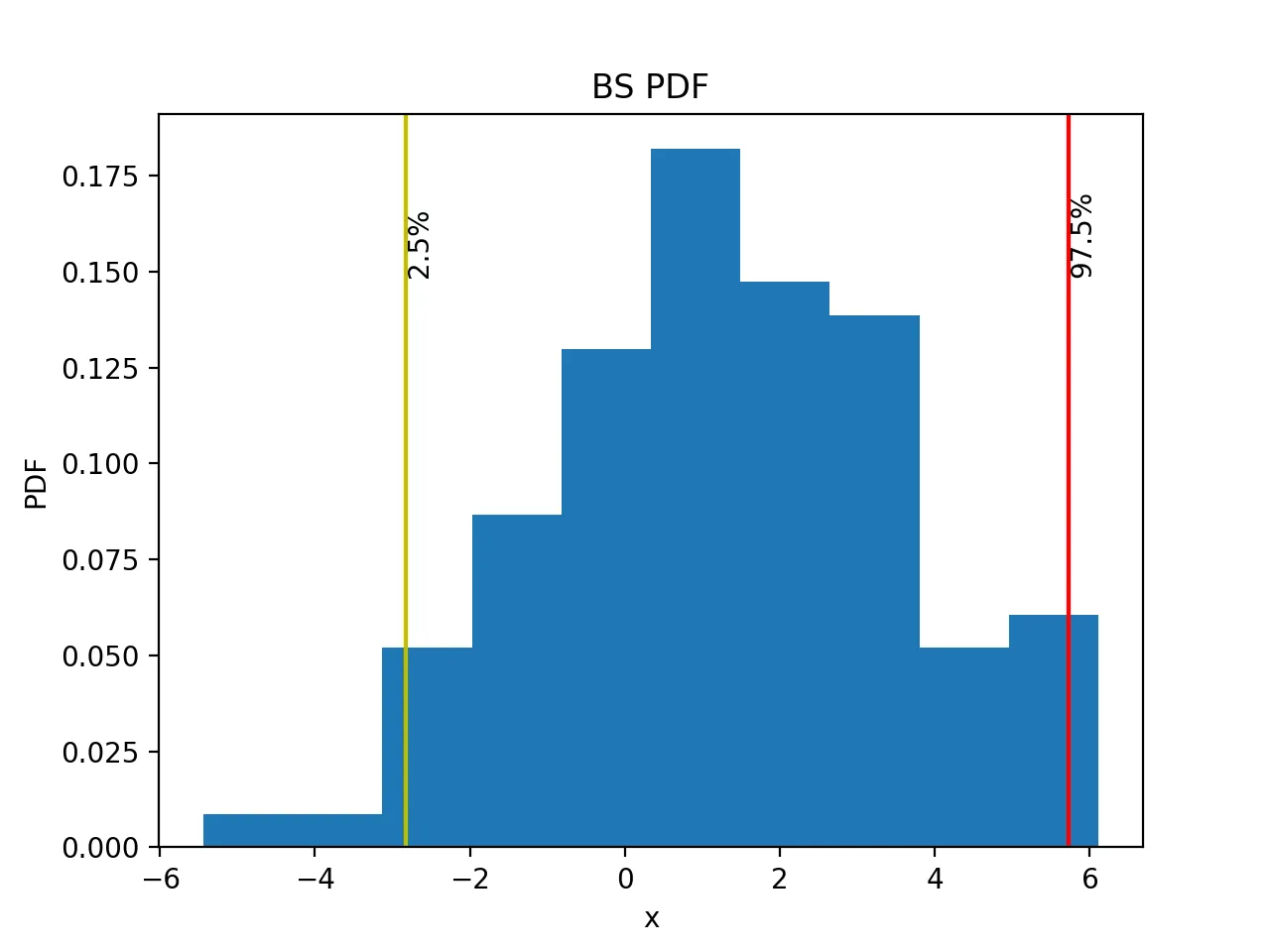
Interpreted correctly, the final interval is the 95% bootstrap confidence interval of the sample mean, not the interval of the last single bootstrap sample.

You can print it directly as well:

print(ci_low, ci_high)

Practical notes

1. Bootstrap resampling should normally be done with replacement, so writing replace=True explicitly is a good habit
2. The percentile step must be applied to the bootstrap statistic you actually care about
3. sns.distplot is an older API; sns.kdeplot or sns.histplot is preferred in newer code
4. Bootstrap is still an approximation, so very small samples or highly unusual distributions need more careful interpretation

Summary

This article introduced the basic idea of confidence intervals and showed, with a Python example, how to use bootstrapping to repeatedly resample a dataset and estimate a 95% confidence interval for the sample mean.

The key point is not just to resample many times, but to be clear about which statistic you are estimating and then compute the percentile interval from the bootstrap distribution of that statistic. Once that part is correct, bootstrap becomes a very practical tool in research and data analysis.